Intrinsic Properties

This example shows how to model the electron transport coefficients in nano-structured silicon.

Band Gap

The following block of code computes the energy range [eV], temperature range [K], and the electronic band gap [eV]:

import ThermoElectric as TE
import numpy as np
from numpy.linalg import norm
from scipy.interpolate import PchipInterpolator as interpolator

energy_min = 0.0  # Minimum energy level [eV]
energy_max = 1  # Maximum energy level [eV]
num_enrg_sample = num_enrg_sample = 4000  # Number of energy points

tmpr_min = 300  # Minimum temperature [K]
tmpr_max = 1300  # Maximum temperature [K]
tmpr_step = 50  # Number of temperature points

engr = TE.energy_range(energy_min = energy_min, energy_max = energy_max,
                       sample_size = num_enrg_sample)
tmpr = TE.temperature(temp_min = tmpr_min, temp_max = tmpr_max, del_temp = tmpr_step)
electronic_gap = TE.band_gap(Eg_o = 1.17, Ao = 4.73e-4, Bo = 636, temp = tmpr)

ThermoElectric uses the following form for the band gap:

\[\mathrm{E_g(T) = E_g(0) - \frac{A_o T^2}{T+B_o}}\]

For the silicon, \(\mathrm{E_g(T) = 1.17\ [eV], A_o = 4.73 \times 10^{-4}\ [eV/K], B_o = 636\ [K]}\), are used. For more details, see “Properties of Advanced Semiconductor Materials” by Michael E. Levinshtein.

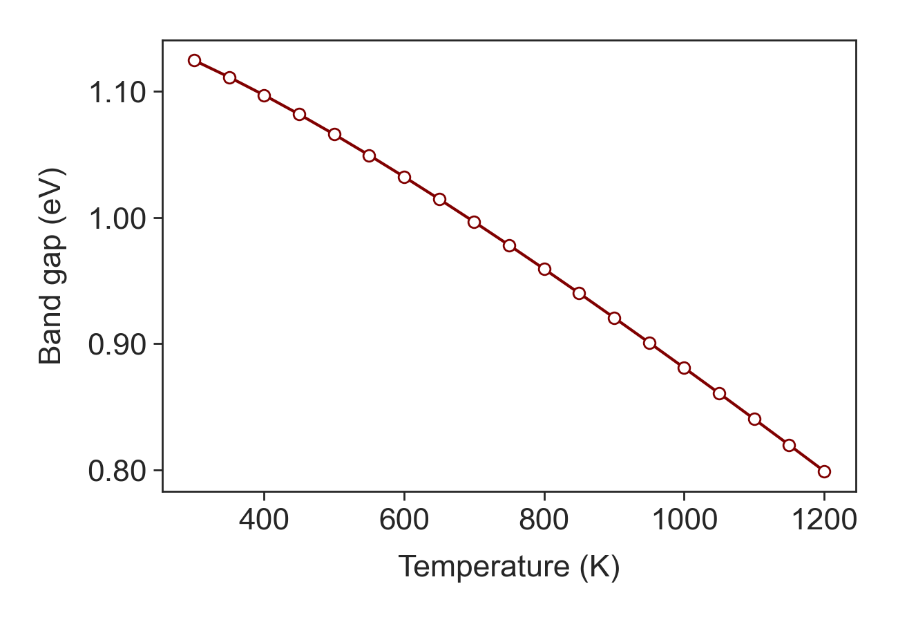
Si band gap.

Next step is to compute total carrier concentration.

Total Carrier Concentration

carrier_con = TE.carrier_concentration(path_extrinsic_carrier =
                                       'Exp_Data/experimental-carrier-concentration-5pct-direction-up.txt',
                                       band_gap = electronic_gap, Ao = 5.3e21, Bo = 3.5e21, temp = tmpr)

The intrinsic carrier concentration is computed using \(\mathrm{N_i = \sqrt{N_c N_v} \exp(\frac{E_g}{2k_B T})}\), where \(\mathrm{N_c = A_o T^{3/2}}\) and \(\mathrm{N_v = B_o T^{3/2}}\) are the effective densities of states in the conduction and valence bands, respectively. For the silicon, \(\mathrm{A_o = 5.3 \times 10^{21}\ [m^{-3}K^{-3/2}], B_o = 3.5 \times 10^{21}\ [m^{-3}K^{-3/2}]}\), are used from “Properties of Advanced Semiconductor Materials” by Michael E. Levinshtein.

Carrier concentration. The solid lines are ThermoElectric predictions. The experimental measurements are marked in black.

We need to define the reciprocal space basis. For Si, the basis is defined as:

lattice_parameter = 5.40e-10  # Si lattice parameter in [m]
lattice_vec = np.array([[1,1,0],[0,1,1],[1,0,1]])*lattice_parameter/2 # lattice vector in [1/m]
a_rp = np.cross(lattice_vec[1], lattice_vec[2])/ np.dot(lattice_vec[0], np.cross(lattice_vec[1], lattice_vec[2]))
b_rp = np.cross(lattice_vec[2], lattice_vec[0])/ np.dot(lattice_vec[1], np.cross(lattice_vec[2], lattice_vec[0]))
c_rp = np.cross(lattice_vec[0], lattice_vec[1])/ np.dot(lattice_vec[2], np.cross(lattice_vec[0], lattice_vec[1]))
recip_lattice_vec = np.array([a_rp, b_rp, c_rp])  # Reciprocal lattice vectors

Next, we compute the band structure [eV], group velocity [m/s], and the density of states (1/m³)

num_kpoints = 800  # Number of kpoints in EIGENVAL
num_dos = 2000 # Number of points in DOSCAR
num_bands = 8  # Number of bands in Si
num_qpoints = 200  # Number of q-points in desired band
valley_idx = 1118  # The index of valley in DOSCAR
unitcell_vol = 2*19.70272e-30 # Silicon unitcell volume

dispersion = TE.band_structure(path_eigen = 'DFT_Data/EIGENVAL', skip_lines = 6, num_bands = num_bands,
                               num_kpoints = num_kpoints)
kp = dispersion['k_points']
band_struc = dispersion['electron_dispersion']

band_dir = band_str[400: 400 + num_qpoints, 4]  # The forth column is the conduction band
min_band = np.argmin(band_dir, axis=0)  # The index of the conduction band valley
max_band = np.argmax(band_dir, axis=0)  # The index of the maximum energy level in the conduction band

kp_rl = 2 * np.pi * kp @ RLv  # Wave-vectors in the reciprocal space
kp_mag = norm(kp_rl, axis=1)  # The magnitude of the wave-vectors
kp_engr = kp_mag[400+max_band: 400+min_band]

energy_kp = band_struc[400+max_band: 400+min_band, 4] - band_str[400+min_band, 4]
sort_enrg = np.argsort(energy_kp, axis=0)
# The electron group velocity
grp_velocity = TE.group_velocity(kpoints = kp_engr[sort_enrg], energy_kp = energy_kp[sort_enrg], energy = engr)
# The electronic density of states
e_density = TE.electron_density(path_density = 'DFT_Data/DOSCAR', header_lines = 6, unitcell_volume= unitcell_vol,
                                num_dos_points = num_dos, valley_point = valley_idx, energy = engr)

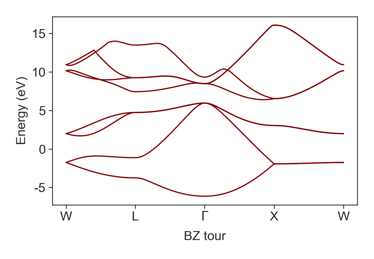
Si band structure.

Fermi Energy Level

We can estimate the Fermi energy level using Joyce Dixon approximation

joyce_dixon = TE.fermi_level(carrier = carrier_con, energy = engr, density = e_density, Nc = None,
                             Ao = 5.3e21, temp = tmpr)

Joyce Dixon approximate the Fermi level using \(\mathrm{E_f = \ln\left(\frac{N_i}{Nc}\right) + \frac{1}{\sqrt{8}} \left(\frac{N_i}{Nc}\right) - (\frac{3}{16} - \frac{\sqrt{3}}{9}) \left(\frac{N_i}{Nc}\right)^2}\).

Next, we are using a self-consistent algorithm to accurately compute the Fermi level.

fermi = TE.fermi_self_consistent(carrier = carrier_con, temp = tmpr, energy= engr, density= e_density,
                                 fermi_levels = joyce_dixon)

Fermi distribution and its derivative (Fermi window) are computed as

k_bolt = 8.617330350e-5  # Boltzmann constant in [eV/K]
fermi_dist = TE.fermi_distribution(energy = engr, fermi_level = fermi[1][np.newaxis, :], temp = tmpr)
np.savetxt("Matlab_Files/Ef.out", fermi[1] / tmpr / k_bolt)

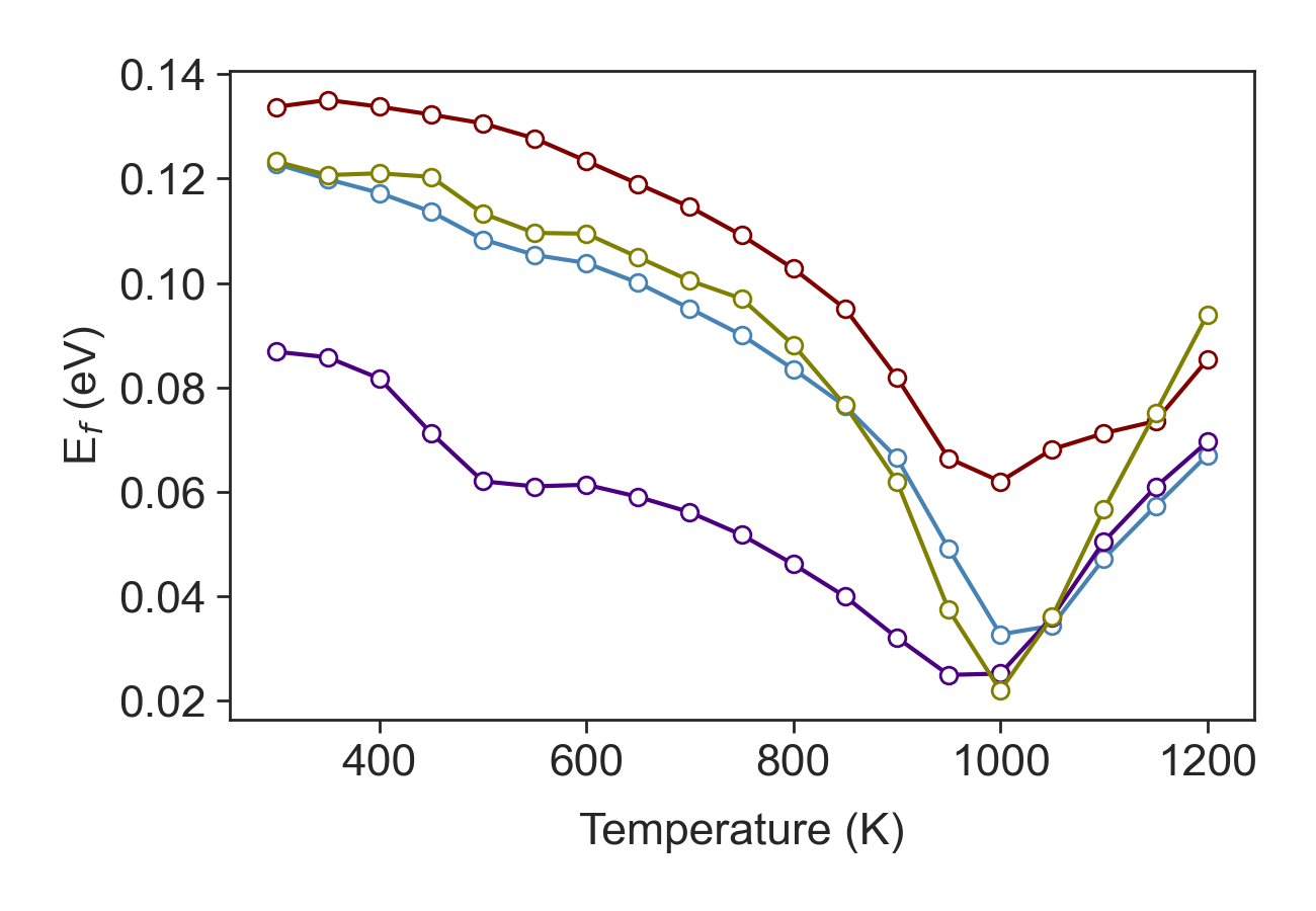
Self-consistent Fermi level calculation.

Generalized Debye Length

We need Ef.out to compute the -0.5-order and 0.5-order Fermi-Dirac integral. The fermi.m is an script writen by Natarajan and Mohankumar that may be used to evaluate the half-order Fermi-Dirac integral integrals. An alternative python tool is dfint

pip install fdint

The generalized Debye length is computed as \(L_D = \frac{e^2 N_c}{4 \pi \epsilon \epsilon_o k_B T }\left[F_{-1/2}(\eta) + \frac{15\alpha k_B T}{4}F_{1/2}(\eta)\right]\)

eps_o = 8.854187817e-12  # Permittivity in vacuum F/m
mass_e = 9.109e-31  # Electron rest mass in Kg
h_bar = 6.582119e-16  # Reduced Planck constant in eV.s
e2C = 1.6021765e-19  # e to Coulomb unit change
nonparabolic_term = 0.5  # Non-parabolic term
dielectric = 11.7  # Relative dielectricity

mass_cond = 0.23 * mass_e * (1 + 5 * nonparabolic_term * k_bolt * tmpr)  # Conduction band effective mass
Nc = 2*(mass_cond * k_bolt * tmpr / h_bar**2 / 2/ np.pi/ e2C)**(3./2)
fermi_ints = np.loadtxt("Matlab_Files/fermi-5pct-dir-up.out", delimiter=',')
screen_len = np.sqrt(1 / (Nc / dielectric / eps_o / k_bolt / tmpr * e2C *
                    (fermi_ints[1] + 15 * nonparabolic_term * k_bolt * tmpr / 4 * fermi_ints[0])))

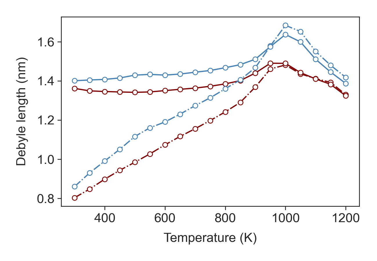
Generalized Debye length.